This post arose because of a discussion with some colleagues about the measurement of utility and health-related quality of life in cancer. It covers latent variable regression and an attempt to use it to describe the relationship between a common measure used to estimate utility (the EQ-5D) and a disease-specific measure of health-related quality of life (the EORTC-QLQ-C30).

‘Eh?’ I hear you saying.

Basically, the problem is: If you have two measures of the same thing, how do you use the information from both of them simultaneously?

The post is about health economic decisions, but the problem generalises to a number of disciplines. WARNING: Here be stats! If you aren’t interested in equations, just skip them.

The majority of regression analyses rely on two or more observed variables with one set of variables, the independent variable(s), used to predict the other set of variables, the dependent variable(s). For example, we may use someone’s height and weight (the independent variables) to estimate their risk of developing diabetes in the next 5 years (the dependent variable).

In this case, the ‘correct’ value of the dependent variable can be known; whatever happens, in 5 years’ time, we will know if each individual has diabetes.

There are, though, many situations where the dependent variable is something intangible, like intelligence, mood or, in health economics work, utility. In this situation, we may want to use multiple variables to estimate an unobserved, or latent, variable.

Latent variable regression is something that is more common in disciplines like psychology and economics where we often talk about hidden features of systems (e.g. intelligence, mood, utility) based on observed data (e.g. exam performance, questionnaire score, or forced choice preference).

Motivating example

A couple of colleagues and I had been working on some data involving quality of life in a particularly nasty cancer. A company was developing a new drug and had, with impressive foresight, decided to include both the EQ-5D and the EORTC-QLQ-C30 as measures of the general health outcome from treatment. Even more handily, both measures were collected simultaneously in their main clinical trial.

These measures produce scores of their own. Typically, these are then used to calculate an estimated health utility score for health economic modelling.

I say the company had foresight. This is because the EQ-5D is a measure preferred by the National Institute for Health and Care Excellence (NICE). As a result, using other measures can cause problems when you try to get the NHS to pay for your drug. However, EQ-5D is often thought to be insensitive to changes in quality of life in cancers, and so a lot of clinicians and researchers prefer a disease-specific measure like the EORTC-QLQ-C30. By including both, the company had covered their bases.

The problem is, each patient will have two scores, an EQ-5D score and an EORTC-QLQ-C30 score. Each of these will produce a utility score. That means there will be two utility scores for each patient, and they will probably be different. Which is right, and how should we reconcile any differences?

It always seems a shame when someone goes to the effort of collecting two measures of, basically, the same thing only to have half the data ignored or, even worse, to have results that may be inconsistent across measures.

Ideally, we would use both measures to get a better estimate of the underlying (i.e. latent) construct quality of life.

Sketching out the problem

I always like to start with a pretty picture of the problem. I think it helps keep things focused. Here it is:

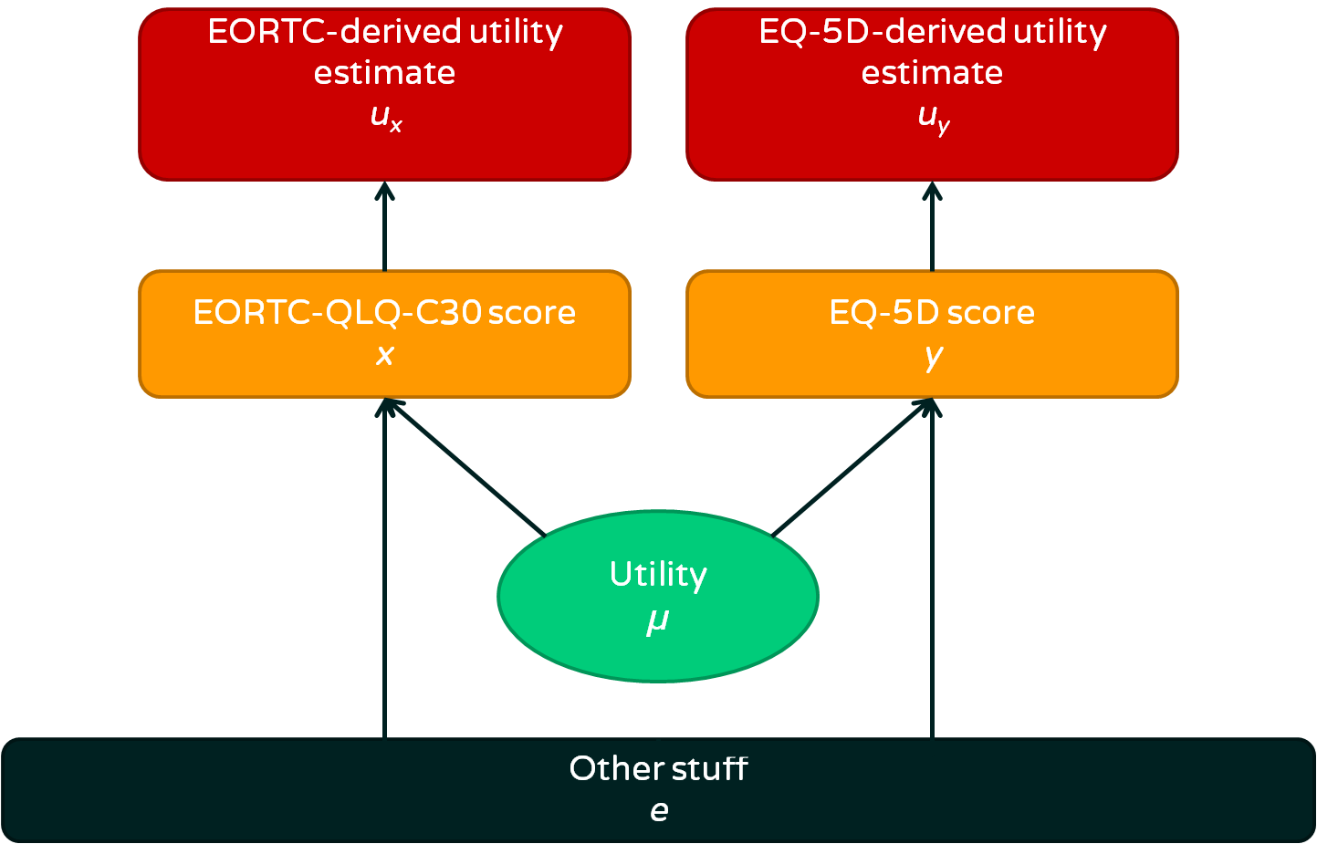
We are interested in utility, which is an abstract concept we can’t measure directly
A person’s utility affects their EORTC-QLQ-C30 and EQ-5D scores
- There is also ‘other stuff’ that affects EORTC and EQ-5D scores, some of it is deliberate and some is measurement error. Overall, we consider this ‘other stuff’ error because it is not directly relevant
We can use calculations to estimate utility from either EORTC or EQ-5D score

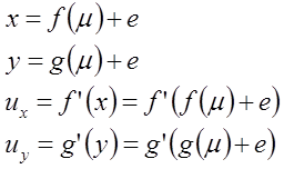
If you prefer to see things as equations, this could be summarised as:

The usual solutions

There are two general approaches taken in this situation:

Choose one of the measures and stick with that as a utility measure, discarding the other measure
Use the more sensitive measure to predict the more standard measure and map between the two

The first approach is understandable in that it keeps things simple. In the case of NICE, the preference would be to ignore the EORTC-QLQ-C30 data and take the EQ-5D estimate. The advantage of this is that the utility measures calculated will be consistent across different diseases because everyone is told to use EQ-5D (normally, at least). This prevents people submitting health economic evidence to NICE from cheating and just choosing whatever measure gives their drug the best chance of success. One disadvantage is that the EQ-5D may not capture utility very well in the population of interest, and so may result in poor decisions being made. A second disadvantage is that a lot of relevant information is lost.

The second approach attempts to deal with the limitations of the first approach by borrowing some of the sensitivity of the EORTC-QLQ-C30 and using it to ‘fill the gaps’ in the EQ-5D measure. To illustrate this, take a look at the graph below (generated using simulated data):

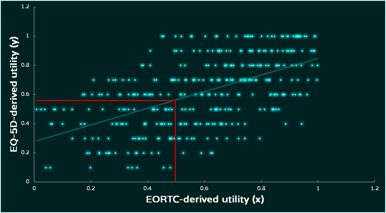
The two utility estimates are regressed, with EORTC-derived utility being used to estimate EQ-5D-derived utility. There are variations on this approach, but the end result is a regression equation that uses the data from both scores. The lack of sensitivty of the EQ-5D is shown by the gaps between different scores on the y-axis. This can be overcome by taking the EORTC-derived score and using the regression equation to calculate the EQ-5D-derived score. There are big gaps between levels in the EQ-5D-derived utility estimate, and a regression line allows us to ‘fill’ those gaps.

This approach has the advantage of allowing a standard scale (the EQ-5D utility) to be used across health technology assessment decisions while making use of all the information collected. One weakness is that it relies on us treating one of the measures as a ‘gold standard’, and that makes me uncomfortable. To my mind, it involves taking an independent variable and treating it as a dependent variable.

The biggest issue, though, is practical. Approaches like this are sensitive to regression assumptions, particularly in assuming that there is enough data available for the regression analysis to reduce uncertainty rather than adding to it. Where the data are lacking, the fit of the regression model may be poor. Utilities have awkward statistical properties and this can make it difficult to work out the source of error.

To summarise, the current approaches are legitimate, but they may not work and they have some fairly serious limitations. With this in mind, I had a play to see what approach I could take.

A direct modelling approach

If we assume that functions f and g are linear and the errors are normally distributed, we can generate a simple statistical model:

(1) $\begin{equation*} \hat{x} = b_{x}\mu + a_{x} \end{equation*}$

(2) $\begin{equation*} \hat{y} = b_{y}\mu + a_{y} \end{equation*}$

Where:

(3) $\begin{equation*} x \sim {Norm}(\hat{x}, s_{x}^{2}) \end{equation*}$

(4) $\begin{equation*} y \sim {Norm}(\hat{y}, s_{y}^{2}) \end{equation*}$

We can actually simplify this a little. If we are submitting to NICE, they will require the result presented on the same scale as the EQ-5D. If we want to force $\mu$ onto the EQ-5D scale, we can adjust (2) so that:

(2.1) $\begin{equation*} \hat{y} = \mu \end{equation*}$

That is not the only scaling adjustment needed. The model above relies on utility being normally distributed, but this is not possible. First of all, utility itself is defined in a way that means it must have an upper bound of 1. While utilities below 0 do occur, for simplicity at the moment, I will assume that utility has a lower bound of 0. In addition, the EORTC-QLQ-C30 is bounded by 0 and 100.

To get around these problems, I will use a relatively simple rescaling trick. This allows us to run the analysis on an unbounded scale (e.g. the normal distribution) and then squash the tails of the distribution to form a bounded distribution.

There may be a neater way of doing it than this, but this is just a prototype for now.

To show how the rescaling trick works and how the latent variable regression works in practice, the table below shows the model, a description of what it means, and BUGS code for the model that could be run in WinBUGS or OpenBUGS.

Model	Description	BUGS code
$x^\prime \sim {Norm}({\hat{x}^\prime}, \sigma^2_{x^\prime})$ $y^\prime \sim {Norm}({\hat{y}^\prime}, \sigma^2_{y^\prime})$ ${\hat{x}^\prime}={b\mu+a}$ ${\hat{y}^\prime}={\mu}$	These are linear models giving expected values for $x^\prime$ and $v^\prime$ given a latent variable $\mu$ . The simultaneous equations are built to place $\mu$ on the same scale as $y^\prime$ . The normal distributions capture error in the estimation. There is no link function because an identity link is used, based on $x^\prime$ and $y^\prime$ being transformed in the next step.	model{ for (i in 1:N){ # Normal likelihood x.prime[i]~dnorm(pred.x.prime[i],tau.x.prime) y.prime[i]~dnorm(pred.y.prime[i],tau.y.prime) # Regression equations (simultaneous) scaled on y pred.x.prime[i] <- b*mu[i] + a pred.y.prime[i] <- mu[i]
${x^\prime}=\log({x \over {100-x}})$ ${y^\prime}=\log({y \over {1-y}})$	$x$ and $y$ are the observed values. These are on different scales and are constrained by their maximum and minimum scores. This part of the code rescales $x$ and $y$ so that they are continuous ratio measures. This approach is based on the logit transformation. The generalised approach to doing this is based on the range of the variable. For example, if a variable $z$ were constrained between a and b: $z \in (a,b)$ it would be transformed to $z^\prime$ as follows: ${z^\prime} = \log{{z-a}\over{b-z}}$	# Rescale observations x.prime[i]<-log(x[i]/(100-x[i])) y.prime[i]<-log(y[i]/(1-y[i])) }
	These are the prior distributions required for a Bayesian analysis.	# Priors for precision tau.x.prime ~ dgamma(1,1) tau.y.prime ~ dgamma(1,1) # Priors for regression parameters b~dnorm(0,1.0E-3) a~dnorm(0,1.0E-3) # Priors for mu for (i in 1:N){ mu[i]~dnorm(0,1.0E-3) }
$\hat{y}={{e^{\hat{y}^\prime}} \over {{e^{\hat{y}^\prime} + 1}}}$	This uses the logistic function to rescale $\hat{y}^\prime$ back on to a scale between 0 and 1 so that it can be interpreted directly as a utility.	# Calculate predicted value for y (estimated utility on EQ-5D scale) for (i in 1:N){ pred.y[i]}}

Summary

Well, that’s the model. It’s just an idea at the moment, and there are probably some mistakes in my thinking. I realise that the content here is probably a bit much for a casual read, so here’s what’s important:

Life is uncertain, so you need to use all the relevant data you have
The statistical methods you learn at school or university (or from your own study) can be restrictive, but it’s possible to come up with new ones
If you do come up with a new approach, test it…

…which brings me to this – If you have any real data where this type of approach may help, maybe we could try it out.

Latent variable regression – an idea

Motivating example

Sketching out the problem

The usual solutions

A direct modelling approach

Summary