Meta-analysis relies on the pooling of data from across studies. This can be a pain because study reports are not usually written with the intention of having their results pooled with other studies. Reports of meta-analyses are sometimes even worse because there are a range of different summary statistics (Hedge’s g, Cohen’s d, odds ratios, risk ratios etc) that may be used.

There are all sorts of modern statistical approaches that allow you to pool data reported using different (but related) measures or the same measure reported in different ways. Things like shared parameter models, multinomial models, and latent variable models allow you to explicitly model the relationship between variables. As a result of this they have, to my mind, a good level of explanatory power and transparency. In other words, it can be clear how they work, so it’s possible for a reader to understand whether they are legitimate.

However, those approaches can be a bit complex. Sometimes, it’s easier to stick with making a few assumptions and converting between different effect measures. Where we have a whole load of different effect measures there are two general approaches we can take:

Back calculate the original data from a summary statistic
Convert different summary statistics into a consistent, common statistic for analysis

Back-calculation

If you have quite a lot of data in a consistent format but just a couple of data points that need converting, the best approach can be back-calculation. This means taking the summary statistic you have and working backwards to try and uncover the data that generated it. The most common situation where this is relevant is where you are trying to do a meta-analysis and the basic data are very similar, but not quite the same. For example, sample means may be reported with varying measures of spread (e.g. standard deviations, standard errors, or confidence intervals).

The general approach to back-calculation is quite simple. Inferential statistics are based on the idea that we have a population of values from which we take a sample and calculate the statistic. That statistic has a sampling distribution. This is simply a distribution that describes how our sample statistic is expected to relate to the underlying population statistic. For example, we may assume that the mean of a sample of data (which we might call $\bar{x}$ ) is randomly related to the population mean (which we might call $\mu$ ) using a normal sampling distribution with standard deviation $\sigma_{\bar{x}}$ . In other words:

(1) $\begin{equation*} \bar{x} \sim Normal(\mu ,\sigma_{\bar{x}}^2) \end{equation*}$

The process for back-calculation is:

Identify the statistic you have and the statistic you want
Identify what values are used to calculate those statistics
Work out what distribution relates the two
On the basis of that, work out how they are related
Make any assumptions needed to back-calculate
Do the sums

An example of back-calculation

Now, let us suppose we are doing an analysis and we want all the data in a consistent format. The studies we are looking at all report the average test score for some children. Here are some data:

Study Name	Mean score ( $\bar{x}$ )	Standard deviation ( $s_x$ )	Standard error ( $s_\bar{x}$ )	Sample size (N)
George (2012)	73	–	5	40
Pearson (2011)	82	24	–	16
Richardson (2014)	71	27	–	85

Our analysis programme likes to use data reported as a mean and standard deviation, so we need to convert the George data to a standard deviation from a standard error.

Identify the statistic you have and the statistic you want – I have a standard error and I want a standard deviation
Identify what values are used to calculate those statistics – The sample standard deviation ( $s_x$ ) is the standard deviation of the distribution from which individual scores are drawn. It is calculated from the scores individual children get.The standard error is an estimate of the standard deviation ( $s$ ) of the distribution from which the mean ( $\bar{x}$ ) is sampled. It is calculated from the mean
Work out what distribution relates the two – In order to calculate a standard error, you assume that the sampling distribution of the mean is normal, so a normal distribution relates the two
On the basis of that, work out how they are related – The shape of the normal distribution is well understood. By looking in some textbooks, we can see that ${s_\bar{x}} = {{s_x} \over {\sqrt{N}}}$ . In other words, as our sample gets bigger, the standard error of the mean gets smaller, which makes sense
Make any assumptions needed to back-calculate – We have to assume that the sample standard deviation is a reasonable estimate of the population standard deviation
Do the sums – ${s_\bar{x}} = {{s_x} \over {\sqrt{N}}}$ , so ${s_x} = {{s_\bar{x}} \times {\sqrt{N}}}$ . Therefore, ${s_x} = {5 \times {\sqrt{40}}} = {{5} \times {6.32}} = {32}$

This is quite an involved process and involves knowing a fair bit about how statistics are calculated. Fortunately, we are often back-calculating between values we understand quite well.

TEST YOURSELF Estimate the standard errors for the Pearson and Richardson studies

Converting between effect measures

This is something that crops up quite a lot in psychological work. For example, different measures of the same quantity (e.g. different algebra exams) may be recorded in different studies.

A common way of collating effects from different studies is to use correlation measures. The logic behind this is that a lot of different statistical comparisons can be thought of as forms of correlation. Let’s look at an example.

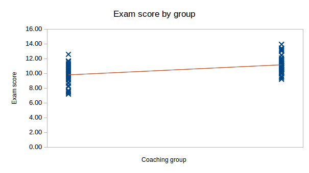
Suppose you want to look at the effect of coaching on exam performance. To do this, you could get two groups and coach one of them, then compare their exam performance at the end. This would be a group comparison, and their results might look like this:

Alternatively, you could get lots of people and give them different amounts of coaching, then record their exam results. The results of this study might look like this:

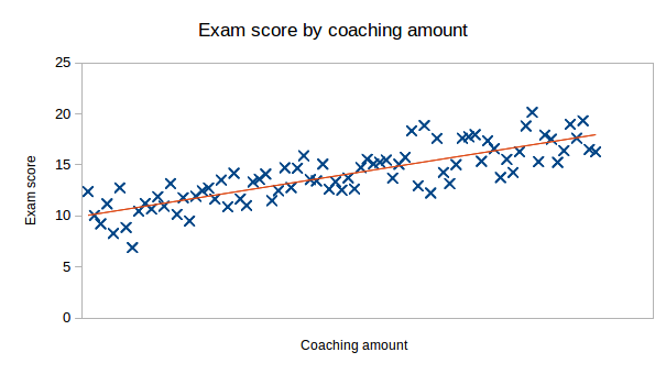
As these plots show, a two group comparison can be treated similarly to a correlation analysis. The important thing is to be able to scale the correlation coefficient appropriately so that the values are truly comparable.

This is very handy because it means that it is possible, with a few assumptions, to convert from a lot of statistics to a correlation measure, $r$ . Some of the most common conversions are shown in the table below, which is heavily based on some material in an excellent book by David Clark-Carter. If you want a broad understanding of statistics for psychology, this is one of the best books I have read, and Clark-Carter gives lots more useful formulae.

Statistic given	Conversion formula	Notes
$t$	${r}={\sqrt{{t^2}\over{{t^2}+{df}}}}$	Watch out for the direction of effect. If appropriate, make $r$ negative.
$F$	${r}={\sqrt{{F_{1,2}}\over{{F_{1,2}}+{df_{error}}}}$	The F-ratio for this has to come from a test with one degree of freedom (i.e. two levels of the variable). This is an ANOVA being used as a t-test. Watch out for the direction of effect. If appropriate, make $r$ negative.
$\chi^2$	${r}={\sqrt{{\chi^2}\over{N}}$	The $\chi^2$ statistics must have one degree of freedom (a 2×2 table). Watch out for the direction of effect. If appropriate, make $r$ negative.
Cohen’s $d$ or Hedge’s $g$ or Glass’s $\Delta$	${r}={{d}\over{\sqrt{{d^2}+{{1}\over{pq}}}}}$	$p$ is the proportion of participants in the experimental group, and $q$ is the proportion of participants in the control group. Watch out for the direction of effect. If appropriate, make $r$ negative.

Summary

While statistics can be reported in a highly variable way, if they are describing the same underlying process there is usually a way of relating them together. If the relationship is comparatively simple, for example an F-test with one degree of freedom or a 2×2 $\chi^2$ test, there’s a good chance that you can describe it using a correlation measure, or any one of the other popular effect size measures (Cohen’s $d$ etc.).

Pooling data that are reported inconsistently

Back-calculation

An example of back-calculation

Converting between effect measures

Summary

Leave a Reply Cancel reply