Meta-analysis is the statistical aggregation of data from a number of studies in order to answer a question. As an example, when considering the efficacy of a treatment, one may pool the results of multiple trials comparing the treatment to placebo.

Originally, meta-analyses involved only direct evidence. That is to say that, when two treatments were compared, only trials involving those two treatments would be included. The logic behind this was clear; if we want to look at the effect of one treatment compared to another, we should use data comparing those two treatments.

For more details on direct meta-analyses, and an example analysis click here.

Unfortunately, the drug development process means that this approach would often lead to delayed assessments of treatments. This has led to some extensions to traditional meta-analysis.

Indirect treatment comparisons

One common frustration that arises with standard meta-analyses is how to interpret indirect data. Often, when investigating the safety or initial efficacy of a treatment, the most appropriate trials would be placebo controlled or against some outdated treatment. Even if trial data are very recent, clinical standards often vary across countries , making it impractical to perform a trial that includes all relevant comparators.

This could result in having to choose between two new treatments that have only ever been compared to placebo and never to one another. For example, let’s imagine that we have a new drug, Monkeyglandin, that we wish to evaluate for the treatment of lycanthropy. When the study was designed, there was no treatment available, so the phase III trial was planned against placebo. Unfortunately (or fortunately if you have lycanthropy), by the time our trial was completed, a new drug called Badgerjuice was in development.

Now that the National Institute for Health and Care Excellence is deciding whether to pay for Monkeyglandin or Badgerjuice, you have no data to compare them directly:

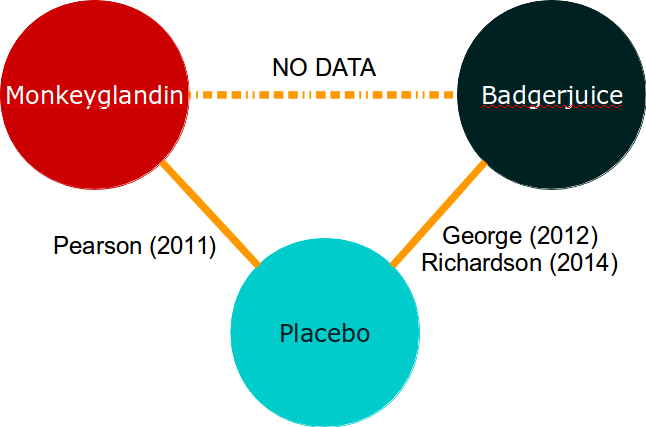Intuitively, when looking at evidence networks like this, one feels that the trial data we do have should allow us to make an informed decision about which treatment is best. Indirect treatment comparisons allow us to do this.

Naively, we may take the observed results from the Monkeyglandin arm of Pearson (2011) and compare them to some pooled estimate from the Badgerjuice arms of George (2012) and Richardson (2014). This approach is possible, but is scientifically and statistically dubious because we cannot differentiate between the differences in outcome due to the treatment used and differences due to differences between the studies.

This is precisely the same issue we had during direct meta-analysis, and the solution is the same: use comparative data.

Essentially, if we use the difference between the active treatment and placebo rather than just taking the results of individual arms, we can remove the study effect from our analyses. This does require the assumption that the study effect is consistent across the arms of the study. However, we have already seen that this is a requirement of direct meta-analysis as well.

To return to our diagram:

The indirect analysis method is based on saying that:

In other words, if we look at the difference between these comparative effects, we can use it to estimate the effect of Monkeyglandin compared to Badgerjuice, because we can effectively adjust for the effect of placebo.

Indirect comparisons introduce uncertainty

When looking at comparative data in direct meta-analysis, we had to add the error variance from each of the arms together because we are, in effect, taking two distributions (the sampling distribution of each treatment arm) and merging them. The same issue occurs with indirect analyses. As a result, the uncertainty around effect estimates from indirect analyses will tend to be larger than that around estimates from direct analyses.

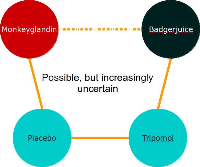
You may see that this principle can be extended to allow indirect comparisons across chains of comparators but that, as evidence chains get longer, the uncertainty around our effect estimate increases pretty quickly.

In summary, indirect meta-analysis is a very simple extension of direct meta-analysis. The assumptions introduced are not really any more severe than for a direct meta-analysis, but they may be more difficult to check because of the complexity of the data. One concern I sometimes have is that any breaches of assumptions may have a bigger effect when they are added across a long evidence chain, particularly if they result in bias. For this reason, I am highly suspicious of long indirect chains of evidence based on the secondary outcomes of trials which can be subject to reporting bias.

Network meta-analysis (NMA) and mixed treatment comparisons (MTC)

We’ve established that one of the advantages of meta-analysis is that it uses more of the available relevant data. We’ve also established that both direct and indirect evidence can be used. Think about that for a moment.

Crikey! Maybe we can use all that data at once!

We certainly can. Analyses across an evidence network are simply an extension of the logic of indirect analyses and direct analyses. They allow us to integrate direct and indirect evidence within a single, coherent analytic framework and, where the data are consistent, they should have more statistical power than either alone.

NOTE: The terminology varies, but the current standard is that network meta-analysis (NMA) refers to any meta-analysis including more than two treatment nodes in the evidence network, while mixed treatment comparison (MTC) involves any analysis where the nodes form a closed loop. On this basis, mixed treatment comparisons and indirect analyses are sub-types of network meta-analysis. Don’t worry about the terminology. Do worry about the evidence networks.

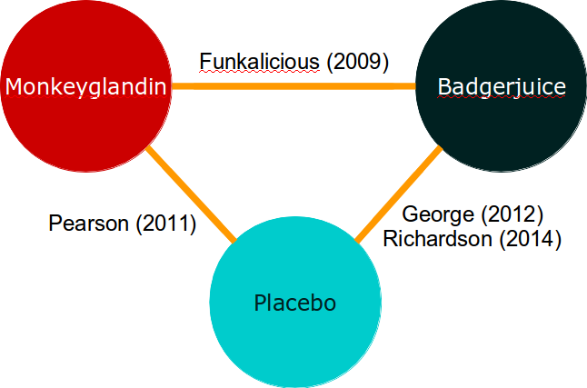
If you’ve worked through the direct meta-analysis example, you can probably even come up with an inverse-variance based method for aggregating direct and indirect evidence. This approach is quite possible for simple evidence networks like this:

However, evidence networks are rather more complex than the nice examples we create for textbooks. A more realistic evidence network might look a bit like this:

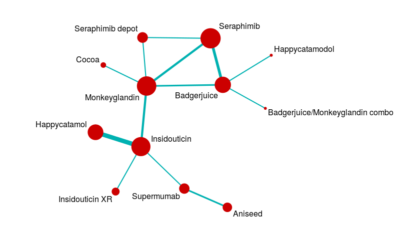
Analysing a network like this is a pretty complicated business, so we usually use statistical packages to help us solve all the simultaneous equations involved.

Issues with mixed treatment comparisons

Back when I first started running mixed treatment comparisons, there was a lot of  discomfort with it. This was a good thing; these methods are pretty complex and it is generally a good idea to be a bit suspicious once an analysis gets so complex that you can’t easily follow all the component parts. Over time, this discomfort has reduced in general. Part of the reason for this is that some great people have worked hard to:

1. Work out what the strengths and weaknesses are
2. Explain those weaknesses in a clear way

I won’t talk about the strengths and weaknesses in detail, but interested readers could do a lot worse than to start here and then read the work of people like Georgia Salanti and Tony Ades or go to some of the courses run by Bristol University and others.

The main issues in mixed treatment comparisons revolve around heterogeneity and consistency. These are a particular issue because complex evidence networks may include ‘archipelagos of uncertainty’. For example, in the complex evidence network above, there is a central mass of data with studies forming closed loops of evidence, but long chains where indirect data predominates. This means that the certainty of our effect estimates will vary across the network. It also means that some of our analyses will involve closed loops, and some will involve open loops.

For closed loops, we can compare the direct and indirect effect estimates to check that nothing funny is happening. This provides some measure of control for subtle biases that can creep in when, for example, the patient group in one part of the network is slightly different from that in another part of the network. When we only have open loops, that check is not available to us. When we have both open and closed loops, we may end up with less confidence in one part of the network than another, and yet the results are driven by data from across the network.

The main advantages of mixed treatment comparisons stem from the same source. Imagine if you did all the analyses within an evidence network separately, and then had to summarise them. You would have done a lot of separate statistical tests, which is dodgy, and the chance of the treatment effect estimates you get being consistent with one another is low. If you wanted to interpret the results to help you choose a single treatment to use out of 5 or 6 available, you would be screwed. Mixed treatment comparisons help you with this problem.

In summary, you need to look at your evidence network and question it before the analysis, but it’s a good idea to synthesise all the available relevant data if you can. Just think carefully about what is relevant.