Meta-analysis
Meta-analysis is the statistical aggregation and analysis of data from multiple studies. When the studies included are properly selected and the data are aggregated appropriately, it uses more of the available information than a single study and so should be more statistically robust.
There are a lot of different methods for meta-analysis, but key issues revolve around the extent to which you weight data from some studies over others (because they are better, or larger, or more credible), the extent to which you can sensibly aggregate data across studies (because of differences between the studies and the people in them, known as heterogeneity), and the methods used to investigate why results differ between studies (e.g. meta-regression).
There are lots of checklists and things that you can use to measure the quality of a meta-analysis. While these have their uses, a checklist without understanding is a dangerous tool for the unthinking. Almost everything that you need to know about a meta-analysis can be derived by having a bit of a think about what causes the data you observe and what that means for how you aggregate the data.
To illustrate that, let’s use an example.
An example
Meta-analysis, like many things, is routinely over-complicated and made to sound like some horrifically complex tool that can only be done by someone more clever than Einstein channelling Newton. That’s nonsense, of course; it’s perfectly possible to do a meta-analysis on the back of an envelope (I suggest using a calculator, though). So let’s do that. As we go through, I’ll point out some main considerations in meta-analysis.
Most of the meta-analyses I do involve trial data, so I will use that as the main example, but do remember that meta-analysis is not just about trials.
When we are looking at the outcome of a clinical trial, such as a study of blood pressure treatments, we may decide that differences in the observed outcome ( – the outcome amongst the patients treated with a particular treatment in a particular study) is a consequence of four things:
- Differences in outcomes between studies (
 ). This is known as the study effect, and may be due to differences in the patients included, the location of the study, and things like that.
 - The effect of the treatment itself (
 ). This is known as the treatment effect and varies because different treatments do different things (we hope!)
 - Differences in the way different patients respond to the drug. I’m going to call this the treatment-study interaction term (
 ). To understand this component, think about trials of paracetamol versus placebo. If some of the trials you are pooling have patients with headaches in them, you would expect to see a treatment effect for paracetamol (
 ). But what if some trials had patients without headaches in them? You would see a difference at the study level, in that the placebo group would have a different effect.
  would take care of this. However, the effect on the response to paracetamol has to be taken care of.
  is involved in this. More on this later.
 - Random measurement errors (
 ).
).
We may decide to put these parameters together in a statistical model. We call them parameters because they are things that we have to infer from observations. We don’t see the study effect directly. Instead, we have to look at and analyse our data in a way that allows us to infer what value it has. The model we use to do this, in this case, looks like this:
(1) 
Pretty much immediately, we can see one major issue if we look carefully at this equation.
Big deal 1 – the assumption of homogeneity of effect
You will notice that both  and have the subscript
  . Remember, we have to work out what the values of our parameters are from our observed data. How on earth are we supposed to differentiate between and if they act in precisely the same way?
Well, we can’t.
 is usually left out of descriptions of meta-analysis. There’s a reason for this – it’s a pain, and it’s bad science to let it get in there. When we are looking at the effect of a treatment, it only really makes sense if we assume that the effect is consistent (or at least sampled from a consistent distribution) across studies. Mathematically, this means that we assume that is 0 and so can safely be ignored.
The way I think of this is to say that we assume that patients from any of the trials would have the same treatment effect if they were switched into a different trial. This is an assumption, so it needs to be checked if possible. It is called, the assumption of homogeneity of effect and, when it is violated, the problem is that we have heterogeneity of effect. It is jargon, but it’s pretty simple jargon and it describes what is going on.
What about ? Doesn’t that have the same problem? Yes and no – this is the next big deal.
Big deal 2 – the assumption that our observations are unbiased
We leave in the equation but, as an error term, we assume that it is a random parameter distributed around 0. If it isn’t distributed around 0, we have bias. This is difficult to check, but can be looked at particularly in meta-analyses with lots of data using things like funnel plots.
The main sources of bias are publication bias and reporting bias. They arise because there are always little random variations in observations of the real world. Sometimes, these will result in a slightly high estimate of  . Sometimes they will result in a slightly low estimate of . If we only include the positive results in our meta-analysis, we will bias our estimate of , and so will not be distributed around 0. This is a huge problem in a world where people have a desire to publish interesting results, as negative results are often not published (resulting in publication bias). My personal concern is that the selective reporting of outcomes is an often underestimated issue, and this results in reporting bias.
The issue of bias is the main reason that robust meta-analysis requires a robust way of identifying evidence. Usually, this means it depends on a well conducted systematic review which has included a systematic assessment of various forms of bias.
Big deal 3 – Use comparative data
Remember that our goal in this example analysis is to investigate treatment effect. In practical terms, this means that we need to get to a situation where we can measure, to some degree of accuracy,  using . If you go back to equation 1, you will see that we have managed to do pretty well. We’ve removed entirely by introducing an analytic assumption, and we’ve controlled the effect of by introducing another assumption and controlling bias. This gives us:
(2) 
We still have , and is a big deal. Studies can vary in many, many ways. Some of those are ways that we can measure, like study duration, some are ways that we don’t measure but can hypothesise, like the way clinicians talk to patients, and some are ways we have never even thought of. The point of this Rumsfeldian spiel is that study effects cannot simply be assumed or wished away. Fortunately, the power of high school algebra is awesome.
If our meta-analysis is of two exciting new treatments, Monkeyglandin and Badgerjuice, that have been investigated in three trials, our evidence network might look like this:
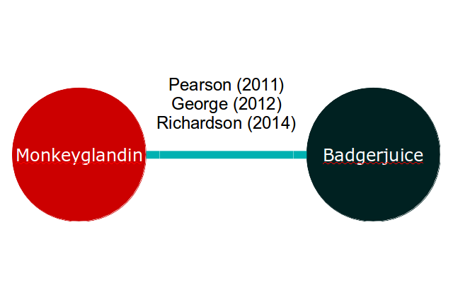 Applying equation 2 to this, we end up with two equations for each study. For example, the George (2012) study results in the following equations:
(3) 
(4) 
Both of these equations contain the parameter  . The magic of high school algebra tells us that we can get rid of this by subtracting one equation from the other:
(5) 
As a result of this, when we do meta-analyses of trial data, we try to use comparative estimates. Without them we can’t reliably distinguish between treatment effects and study effects, and that’s a big deal.
Big deal 4 – Not all studies are equal
We haven’t quite finished with the error terms. If you look at equation 5, you’ll see that there are two terms. Earlier on, I said that we need to assume that these terms are randomly distributed around 0. I think some actual data would make this bit easier, so let’s look at the (fictitious) results from our (fictitious) studies. If Monkeyglandin and Badgerjuice are blood pressure treatments, our outcome measure may be mean change in blood pressure. Blood pressure is usually measured in millimetres of mercury (mmHg). Here are the data:
| Study Name | Monkeyglandin | Badgerjuice | ||||
|---|---|---|---|---|---|---|
| Mean change in blood pressure (mmHg) | Standard deviation | N | Mean change in blood pressure (mmHg) | Standard deviation | N | |
| George (2012) | 4.90 | 4.02 | 100 | 0.77 | 4.29 | 100 |
| Pearson (2011) | 4.55 | 4.16 | 350 | 0.80 | 3.87 | 350 |
| Richardson (2014) | 5.40 | 3.53 | 50 | 0.52 | 3.86 | 50 |
The goal of our meta-analysis is to create a pooled estimate from these data. That is, we want to create an estimate of the difference between Monkeyglandin and Badgerjuice using all the data here. We could just take a simple average. For the data here, that would mean adding up the difference in change scores and dividing by 3:
![\[ \frac{(4.90-0.77)+(4.55-0.80)+(5.40-0.52)}{3}=\frac{12.76}{3}=4.25 \]](https://monkeyglandin.com/wp-content/ql-cache/quicklatex.com-813550be2d400abc66feb776e599f205_l3.png "Rendered by QuickLaTeX.com")
There is a problem with this, though. Look again at those studies. How big are they?
The Pearson study is seven times the size of the Richardson study. Surely, it should count for more.
Indeed it should, and the clue is in our statistical model:
(6) 
Those values are staring at us, daring us to do something with them.
Remember, they are error terms. What they are telling us is that, when we use  to estimate
  , our measurement error means we are wrong by
  .
.
Our results are aggregate values. In this case, we are using mean estimates from a (presumably) normal distribution. Therefore, is an error in the estimate of the mean. The mean error in the estimate of the mean is the standard error, and the total error is the variance of the sampling distribution (which is the standard error squared). Our equation tells us that our estimate of the difference between the two treatment arms for each study is off by the variance of the Monkeyglandin mean plus the variance of the Badgerjuice mean. It may not be obvious why the variances are added when the values are subtracted. The answer is that we are adding up distributions rather than values and, because of this, we are using something called the variance sum law (the links contain the equations, so I won’t repeat them here).
If we apply this, we get the following results for our three studies:
| Study | Mean difference in effect between Monkeyglandin and Badgerjuice | Variance of the difference | Standard error of the difference | Inverse variance |
|---|---|---|---|---|
| George (2012) | 4.13 | 0.35 | 0.59 | 2.89 |
| Pearson (2011) | 3.75 | 0.09 | 0.30 | 10.84 |
| Richardson (2014) | 4.88 | 0.55 | 0.74 | 1.83 |
This shows us two things:
- The studies differ in how well they estimate the true difference in treatment effects
- That inaccuracy can be estimated
It follows that we should probably use that knowledge to adjust how we use the data. This is something we call weighting.
That bit did require some basic statistical knowledge. If it made no sense, fear not. The online statbook has one of the best demonstrations of the relationship between a standard deviation and a standard error I have seen. The best explanation of variance and why we use standard deviations and standard errors that I have ever seen is in Howell’s Statistical Methods for Psychology, which also has some great online material.
The summary is that a standard deviation is the average size that a value within a population varies from the mean of that population. If we take lots of samples of the same size from this population and calculate a mean for each of those samples we eventually get a sampling distribution. The standard error is the standard deviation of this sampling distribution. It tells us the average error of an estimate of the mean. What is really nifty is that we can use the amazing power of the central limit theorem to estimate our standard error from a standard deviation as long as we know the size of our sample.
Understanding sampling distributions is vital to understanding statistics generally, so I suggest reading up on it if any of that doesn’t make sense. When I get a chance, I’ll put together a post describing it in detail with pretty pictures. I like pretty pictures.
Big deal 5 – Use weighting to deal with the inequality of studies
There’s a column in the table above called inverse variance. As the sample size gets larger, the variance decreases. One way to use this to weight studies is to use an inverse variance method, whereby we weight each study by the inverse of its variance (i.e.  ). The smaller the variance, the larger the inverse variance, and so the more weight the study provides to the analysis.
To use inverse weighting, we simply multiply each result by its weight, add them up, then divide by the total weight:
![\[ Pooled \, estimate = \frac{(4.13 \times 2.89) + (3.75 \times 10.84) + (4.88 \times 1.83)}{2.89 + 10.84 + 1.83} = 3.95 \]](https://monkeyglandin.com/wp-content/ql-cache/quicklatex.com-15ee35588db6e422b0b09660260dc8ff_l3.png "Rendered by QuickLaTeX.com")
We can even work out the standard error by adding up the weights and square rooting the inverse of the result:
![\[ Standard \,error\, of\, the\, estimate = \sqrt{{1}\over{2.89 + 10.84 + 1.83}} = 0.251 \]](https://monkeyglandin.com/wp-content/ql-cache/quicklatex.com-dc42e9af60e9b3ea051f52a8dd3eb87d_l3.png "Rendered by QuickLaTeX.com")
We can use the standard error to express our findings as a point estimate and 95% confidence interval. In this case, the mean difference in effect between Monkeyglandin and Badgerjuice is 3.95 mmHg (95%CI: 3.46-4.44).
You may be interested to know that I created the data by simulating data from real distributions. The real underlying population difference in means was 4 mmHg with a standard deviation of 1, so our meta-analysis has done pretty well, and has certainly done better than just taking an average.
If you want to have a go at doing some analyses yourself, here’s a simple meta-analysis workbook that will do an inverse variance weighted analysis for you. Do let me know if it’s useful.
Weighting studies using inverse variance and related measures is not the only way of accounting for the varying certainty different studies provide. For example, if your studies are the same size, but differ markedly in quality, you may decide to weight their influence using some quality measure. The problem with these approaches is that you need to justify both the general approach and the specific weighting you use. You also need to check how sensitive your results are to the weighting approach you have used. Tricky, but sometimes worthwhile.
Summary
Meta-analysis is not trivially easy, but it is logical and understandable with some basic effort. All meta-analytic models introduce some assumptions, and all meta-analytic models can be misused. This makes them precisely as complex as any other statistical model, and no more so.
A note
I don’t actually like the definition of meta-analysis I’ve given here. It is historically accurate, but I tend to think that non-statistical aggregation of data across studies is equally useful, and that all synthesis of data across studies is meta-analysis or meta-synthesis, and that the statistics stuff is a method within this. I doubt anyone would agree with me on that, and it doesn’t really matter. What does matter is that you know that you can combine information across studies even when the data are of a type that doesn’t really fit a statistical modelling approach.
If you want to look at methods like meta-ethnography, there’s lots of material available, including some nice introductory material. In general, I would suggest not worrying about the jargon and just thinking:
- Is it likely that someone has looked at this before? If so, search for and synthesise the evidence
- To figure out how to synthesise the evidence, just sketch out on a piece of paper what you are interested in and what causes it. For example, you may be interested in health outcomes which are caused by a disease process, which is in turn affected by patient features and treatment. Alternatively, you may be interested in the words people use to describe their health and those may be caused by the person’s linguistic background and style as well as their feelings about health. This is a model. Then have a think about whether that model looks like it can be explained best using numbers or a different approach. If in doubt, have a chat with someone
- If you think your model has bits that are statistical and bits that aren’t, great. You’re probably doing something really interesting. Discuss it generally, and have a go at doing a bit of both but please, please don’t overcomplicate things. If you invent a new jargon to explain what you’re doing, you’re making it too complex
Leave a Reply
You must be logged in to post a comment.